Introduction: The Order in Which Groundwater “Decays” (Reduces)
As river water infiltrates underground and flows through an aquifer over decades, its chemical composition changes dramatically.
What drives this change is organic carbon. As microorganisms decompose organic matter, they utilize “electron acceptors” in a specific sequence. This sequence is governed by thermodynamic inevitability.
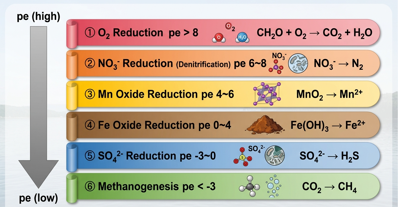
O₂ provides the highest energy yield, so it is consumed first. It is followed by NO₃⁻, Mn oxides, Fe oxides, SO₄²⁻, and finally CO₂ (producing CH₄).
This sequence manifests both spatially (along the flow path in the aquifer) and temporally (in the history of burial and deposition).
The conceptual diagram at the beginning of this article (Appelo & Postma, 1996) illustrates how these “waves” appear one after another. In this session, we will calculate this sequence using PHREEQC.
- The thermodynamic order of redox reactions and the pe–pH relationship
- How to progressively oxidize organic carbon using the
REACTIONblock - Tracking simultaneous changes in O₂, NO₃⁻, Mn²⁺, Fe²⁺, SO₄²⁻, and CH₄ concentrations
- Simulating the spatial Redox front with the
TRANSPORTblock - Reproducing the Appelo & Postma diagram using Python
Theory: Thermodynamic Order of Redox Reactions
Half-Reactions and Gibbs Energy
If we arrange the reduction half-reactions of each electron acceptor by the Gibbs energy ΔG° gained (kJ/mol CH₂O), we get the following sequence:
| Order | Reaction (Oxidation of CH₂O) | ΔG° (kJ/mol) | Environment |
|---|---|---|---|
| ① | CH₂O + O₂ → CO₂ + H₂O | −479 | Oxic |
| ② | CH₂O + 4/5 NO₃⁻ + 4/5 H⁺ → CO₂ + 2/5 N₂ + 7/5 H₂O | −453 | Denitrification (Suboxic) |
| ③ | CH₂O + 2MnO₂ + 4H⁺ → CO₂ + 2Mn²⁺ + 3H₂O | −349 | Mn reduction |
| ④ | CH₂O + 4Fe(OH)₃ + 8H⁺ → CO₂ + 4Fe²⁺ + 11H₂O | −114 | Fe reduction (Suboxic-Reducing) |
| ⑤ | 2CH₂O + SO₄²⁻ → 2CO₂ + H₂S + 2H₂O | −96 | Sulfate reduction (Reducing) |
| ⑥ | 2CH₂O → CO₂ + CH₄ | −58 | Methanogenesis (Strongly Reducing) |
The larger the absolute value of ΔG°, the more “profitable” the reaction is. Therefore, microorganisms utilize them in the order from ① to ⑥. This is the thermodynamic basis for redox sequences.
Correspondence with the pe–pH Diagram
Each reaction is sequentially activated as pe (the negative logarithm of electron activity) decreases:
PHREEQC Code
Before Reading the Code: The Role of the 4 Blocks
containing O₂, NO₃⁻, and SO₄²⁻.
pe = 4 represents a "moderately oxidizing" state.
When carbon is added, they dissolve
and release Fe²⁺ and Mn²⁺.
With each addition, pe drops,
and TEAs (Terminal Electron Acceptors) are sequentially consumed.
to display concentration changes
in real-time during execution.
Full Code
KNOBS
    -step_size 10
    -pe_step_size 5
    -diagonal_scale true
SOLUTION 1
    temp      25
    pH        6
    pe        4
    redox     pe
    units     mmol/kgw
    density   1
    Na        1.236
    K         0.041
    Mg        0.115
    Ca        0.067
    Cl        1.467
    N(5)      0.058
    S(6)      0.085
    Alkalinity 0.26
    O(0)      0.124
    -water    1 # kg
EQUILIBRIUM_PHASES 1
    Goethite  0 0.0025
    Pyrolusite 0 4e-005
    FeS(ppt)  0 0
REACTION 1
    C          1
    0.572 millimoles in 26 steps
INCREMENTAL_REACTIONS True
USER_GRAPH 1
    -headings               C O2 NO3 Mn(+2) Fe(+2) SO4 S(-2) CH4
    -axis_titles            "Carbon added (mmol/kg)" "Concentration (mol/kg)" ""
    -initial_solutions      false
    -connect_simulations    true
    -plot_concentration_vs  x
  -start
10 graph_x step_no*0.572/26
20 graph_y tot("O(0)")/2, tot("N(5)"), tot("Mn(2)"), tot("Fe(2)"), tot("S(6)"), tot("S(-2)"), tot("C(-4)")
  -end
    -active                 true
END
Meaning of Each Section
SOLUTION — Initial Solution
| Line | Meaning | Note |
|---|---|---|
| pH 6 / pe 4 | Slightly acidic, moderately oxidizing | pe=4 corresponds to an aquifer where O₂ is still present |
| units mmol/kgw | Sets concentration units to mmol/kgw | All subsequent values are interpreted in this unit |
| O(0) 0.124 | Dissolved O₂ ≈ 2 mg/L | O(0) is by atomic weight of O. O₂ = O(0)/2 = 0.062 mmol |
| N(5) 0.058 | NO₃⁻ ≈ 3.6 mg/L | N(5) = Nitrogen with oxidation state +5 = Nitrate nitrogen |
| S(6) 0.085 | SO₄²⁻ ≈ 8.2 mg/L | S(6) = Sulfur with oxidation state +6 = Sulfate sulfur |
EQUILIBRIUM_PHASES — Solid Phases
| Mineral Name | Formula | Initial Moles | Role |
|---|---|---|---|
| Goethite | FeOOH | 0.0025 | Dissolves in the Fe-reducing zone to release Fe²⁺ |
| Pyrolusite | MnO₂ | 4×10⁻⁵ | Dissolves in the Mn-reducing zone to release Mn²⁺ (small amount) |
| FeS(ppt) | FeS | 0 | Acts as a sink where H₂S (from sulfate reduction) and Fe²⁺ precipitate |
FeS(ppt) 0 0
The first 0 is the target saturation index (SI = 0 = equilibrium), and the second 0 is the initial amount (moles). Setting the initial amount to zero means “this mineral doesn’t exist initially, but it is allowed to precipitate if it becomes oversaturated”. When H₂S is produced during sulfate reduction, it reacts with Fe²⁺ and precipitates as FeS, effectively removing Fe²⁺ and S²⁻ from the solution.
REACTION and USER_GRAPH
C 1 declares that carbon (C) is used as the reactant. 0.572 millimoles in 26 steps means a total of 0.572 mmol is divided into 26 equal steps, meaning about 0.022 mmol of carbon is added per step.
The equation for graph_x, step_no * 0.572/26, converts the step number into “added carbon amount (mmol)”. Note that tot("O(0)")/2 divides the total atomic O by 2 to convert it to molecular O₂.
In simulations where the electron state changes rapidly—especially during nitrogen reduction—PHREEQC’s calculations often fail to converge and result in an error. By adding a KNOBS block at the beginning of the code and configuring parameters like -step_size 10 or -pe_step_size 5 (which limit the maximum allowable pe change per step), the calculation is stabilized and can successfully run to completion.
How to Read the Calculation Results
The X-axis represents the “Carbon added (mmol/kg)”, ranging from 0 to 0.572 mmol. As carbon increases, each electron acceptor changes in sequence.
| Stage | Approx. Carbon Added | Observed Change | Geological/Environmental Context |
|---|---|---|---|
| ① O₂ Consumption | 0 → 0.06 mmol | O₂ drops rapidly. The O(0)/2 curve is the first to fall. | Recharge zone from river to groundwater |
| ② NO₃⁻ Consumption | 0.06 → 0.13 mmol | NO₃⁻ decreases. The drop in pe temporarily slows down. | Nitrate disappearance in deep groundwater under agricultural areas |
| ③ Mn²⁺ Appearance | Around 0.13 mmol | Pyrolusite dissolves, leading to a spike in Mn²⁺ (short-lived due to small amounts). | Causes Mn issues in aging wells |
| ④ Fe²⁺ Appearance | 0.15 → 0.40 mmol | Goethite dissolves, increasing Fe²⁺. This represents the largest solid phase. | Reddish-brown well water and pipe scaling |
| ⑤ H₂S Generation | 0.40 → 0.57 mmol | SO₄²⁻ drops; H₂S appears. Fe²⁺ is scavenged by FeS(ppt). | Sulfur smell in hot springs or old oil field brines |
| ⑥ CH₄ Generation | After 0.57 mmol | C(-4) = CH₄ appears. Starts only after all TEAs are depleted. | Wetlands, peat bogs, deep coal seams |
Correspondence with Appelo & Postma’s Diagram
The reason the “waves appear to overlap” in the opening figure is because the concentration changes of each component exhibit peaks:
once the reaction begins.
They form the "left half of a wave".
but get consumed again or precipitate
in subsequent reactions, forming the "right half of a wave".
Fe²⁺ appears twice on the right edge of the graph. This is due to:
- The first peak: Generation of Fe²⁺ from the reductive dissolution of Goethite (pe 0 to 4).
- The second increase: In the strongly reducing zone (pe < −3), once SO₄²⁻ is converted to H₂S, the dissolution of Fe²⁺ exceeds the precipitation of FeS₂ (pyrite).
If we check the SI of pyrite in PHREEQC, we can confirm this behavior computationally.
Conclusion
Microorganisms maximize energy.
along the flow distance
and depth in sediments.
are direct indicators of
the current redox stage.
We will input actual water quality analysis data (from an upstream and a downstream point) and reverse-engineer how much of which mineral dissolved or precipitated between them. The types of reactions learned in Redox sequences will serve as the “candidate reaction list” for inverse modeling.
References
Other articles in this series:
- #1 Installation and Initial Calculation
- #2 Analyzing Seawater with Speciation
- #3 Mineral Equilibrium and Temperature Effects
- #4 Calcite–CO₂ Interaction (Open vs. Closed Systems)
- #5 Mixing Groundwater and Seawater
- #6 Pyrite Oxidation and AMD Formation
- #7 Solubility Diagrams (Gibbsite)
- #8 Visualization with Python
- #9 Ionic Strength and Activity Coefficients
- #10 Mastering the Saturation Index (SI)
- #11 Reaction Path Modeling
- #12 Advection-Dispersion Model
- #13 Redox Sequences — The Order of Groundwater Reduction
- #14 Inverse Modeling — Estimating Reactions from Field Data (Coming Soon)
DeepFlow | Science beneath the surface